
Why lateral dimensions can be determined much more precisely than pixel size
Summary
In industrial image processing, it is often assumed: “A pixel is the smallest measurable lateral unit.” This is true for pure pixel counting—but not for determining the position of edges, lines, or centers. Through subpixel evaluation, the position of an edge between pixel centers can be determined more accurately. This application note uses a real-world example to show how, despite a lateral pixel size of approx. 30 µm x 30 µm, a repeatability of 2–3 µm is achieved (typically ~1/10th of a pixel under suitable conditions).
1. Motivation
Many users derive the measurement limit directly from the pixel size:
- Pixel size = smallest lateral measurement
- “Subpixel” sounds like “magic”
The crucial point is: Edges are not imaged by optics, sensors, and lighting as a sharp step change on exactly one pixel, but as a transition across several pixels. It is precisely this transition profile that contains the information needed to determine a position between pixel centers.
2. Basic Principle: Why subpixel is possible
If an edge does not run exactly through pixel centers, its intensity is distributed over several neighboring pixels. This creates a brightness gradient (transition profile) across multiple pixels.
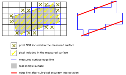
Figure 1: Principle of subpixel-accurate edge determination
Instead of determining the “pixel index of the step,” the edge position is estimated as a continuous parameter—e.g., by:
- Interpolation around the gradient maximum (1D/2D)
- Fitting a model to the edge profile (e.g., sigmoid/error function)
- Geometric fit (line/circle) to many subpixel edge points (Least Squares)
Important: Subpixel does not mean “arbitrarily accurate.” The achievable precision is limited by, among other things:
- Signal-to-Noise Ratio (SNR)
- Bit depth / quantization
- Optics (MTF), focus, motion
- Contrast & lighting (avoid saturation)
- Model/fit bias (systematic deviations)
Practical rule of thumb: Under good conditions, factors of 5× to 10× compared to “pixel accuracy” are realistic.
3. Measurement Object and Setup
3.1 Measurement Object
A PCB connector DFMC 1.5/3-ST-3.5 (© Phoenix Contact) with 6 round cavities serves as an example.
- Nominal diameter: Ø 3.0 mm
- Tolerance: ± 50 µm (LSL = 2.95 mm, USL = 3.05 mm)
Goal:
- Repeatability of diameter determination
- Demonstration of subpixel capability in practice
3.2 Measurement System
- heliInspect™ H9S 0.8× with S40U sensor
- Lighting: Red LED
- Mechanics: Mounted on heliProfiler™ P4
- Evaluation: Contour detection + circle fit (Least Squares / RLS)
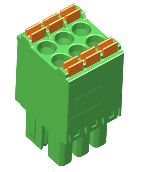
Figure 2: Measurement object (connector) and measurement setup/view of the cavities
4. Data Acquisition and Evaluation
4.1 3D Data and ROI Selection
For contour analysis, only areas with sufficient signal are evaluated (above the noise level). The six cavities are selected as ROIs.
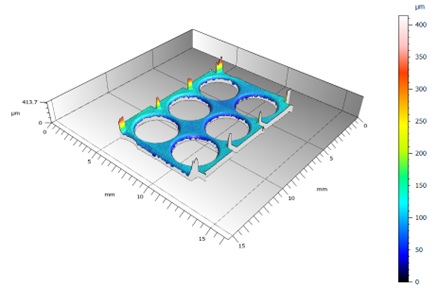
Figure 3: Raw contour/edge points – pixel grid discretization is visible
4.2 Subpixel Edge Points and Circle Fit
In the next step, subpixel edge points are determined and a circle fit is performed over many points. Even if individual points are only “slightly subpixelated,” the combination of many points significantly stabilizes the estimate.
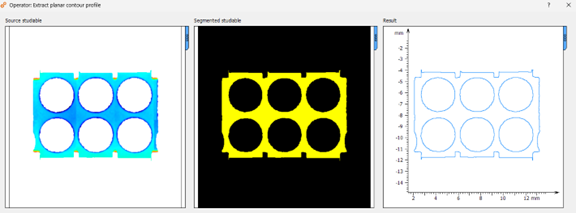
Figure 4: Best-fit circle (Least Squares/RLS) over the contour points
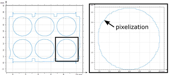
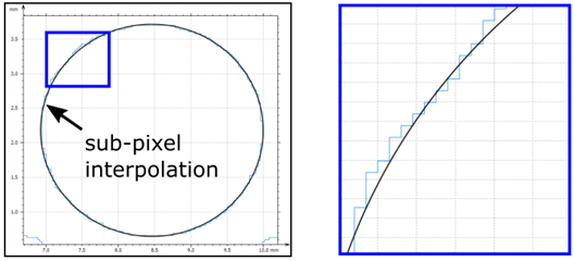
Figure 5: Detail: Raw contour (pixelated) vs. fit (smooth) – subpixel principle of operation.
5. Results: Repeatability
5.1 Measurement Plan
- 30 repetitions at the same location
- Evaluation of the 6 cavities per image
- Parameters: Mean (µ) and standard deviation (σ) of the diameters
5.2 Results
Combined across all cavities and repetitions, the results are:
- Mean: µ = 3.043 mm
- Standard deviation: σ = 0.0025 mm = 2.5 µm
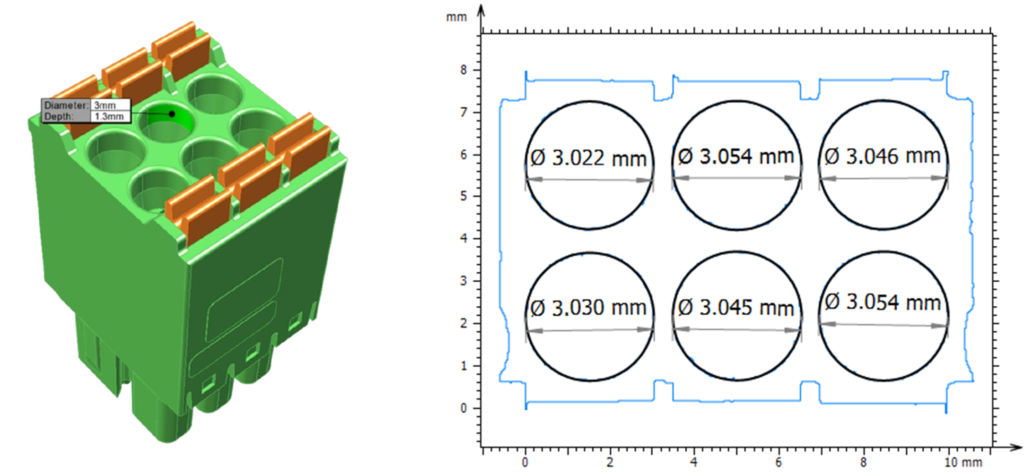
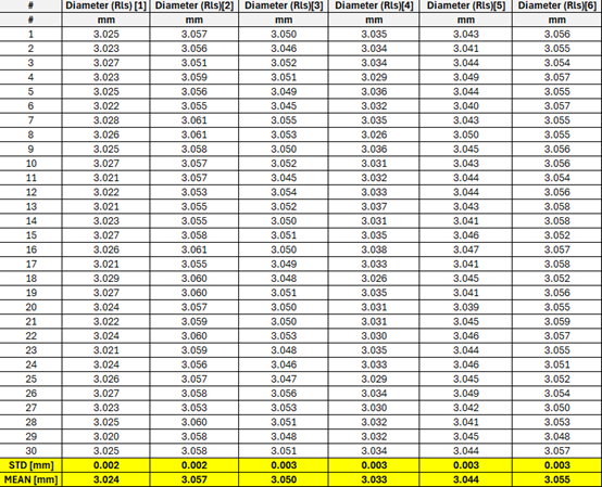
Figure 6: Measured values per cavity over 30 repetitions
Findings:
- Variation in the range of 2–3 µm is consistent with “~1/10th pixel” at ~30 µm pixel size.
- The mean value is close to the upper specification limit (USL = 3.05 mm). This is relevant for Cp/Cpk.
6. Process Capability Indices Cg and Cgk
The indices Cp/Cpk are used here to categorize the measurement variation in relation to the tolerance and the position of the mean.
6.1 Definitions
Cg → “How wide is the tolerance in relation to the variation?”
Cgk → “How much usable tolerance remains, considering the actual process position?”
6.2 Inserting the Values
- LSL = 2.95 mm
- USL = 3.05 mm
- Tolerance width = 0.10 mm
- σ = 0.0025 mm ⇒ 6σ = 0.015 mm, 3σ = 0.0075 mm
- µ = 3.043 mm
Cg:
Cp = 0.10 / 0.015 ≈ 6.67
Cgk:
(USL − µ) / (3σ) = (3.05 − 3.043) / 0.0075 ≈ 0.93
(µ − LSL) / (3σ) = (3.043 − 2.95) / 0.0075 ≈ 12.4
Cgk = min(0.93; 12.4) = 0.93
6.3 Interpretation
- Cg very high: The variation is very small in relation to the tolerance → very precise measurement.
- Cgk significantly smaller than Cg: The mean is close to USL. This does not indicate “too much noise,” but rather positioning/offset (e.g., real component slightly oversize, calibration, thresholds, fit bias).
7. Practical Tips: How to reliably achieve subpixel performance
Subpixel accuracy comes from good imaging conditions—not from “magic”:
- High, stable contrast at the edge (no flare artifacts)
- No saturation (do not clip profiles)
- Good focus / stable optics (MTF)
- Good SNR (appropriate exposure, stable lighting)
- Robust fit (sufficient points, plausible model)
- Constant evaluation parameters (otherwise the bias drifts)
8. Conclusion
This example shows why lateral measurements are not limited to pixel size: By distributing the signal over several pixels, the position of edges and geometries derived from them can be determined at a subpixel level. In the measurement series, we achieve a repeatability of σ ≈ 2.5 µm, even though the lateral pixel size is approximately 30 µm.
The lateral pixel size is not the physical limit of measurement accuracy—it is merely the sampling basis of a continuous signal.
 Heliotis AG